Options

The options toolkit is built on one idea: the Black–Scholes price is a plain differentiable JAX function, so every Greek is an autodiff derivative of it. There are no hand-coded Greek formulas to drift out of sync with the pricer, and the same vmap that prices a chain also differentiates it.

Pricing

black_scholes_price prices a European option. Every array argument broadcasts, so it prices whole chains at once. The convention is a boolean is_call.

from jaxfolio.options import black_scholes_price

# ATM 3-month call, 20% vol, 3% rate
price = float(black_scholes_price(spot=100.0, strike=100.0, ttm=0.25,
                                  vol=0.20, rate=0.03, is_call=True))

Argument	Meaning
spot, strike	underlying price and strike
ttm	time to maturity, in years
vol	annualized volatility
rate, div	continuous risk-free rate and dividend yield
is_call	True for a call, False for a put

For American-style options, binomial_american runs a Cox–Ross–Rubinstein lattice with early-exercise checks at every node (steps controls resolution).

Implied volatility

implied_volatility recovers vol from a market price via jitted Newton iterations — and the vega in the Newton step is itself jax.grad of the pricer, so no derivative is hand-written:

from jaxfolio.options import implied_volatility

iv = float(implied_volatility(price, spot=100.0, strike=100.0, ttm=0.25, rate=0.03))
# ≈ 0.20 — recovers the vol that produced `price`

Greeks via autodiff

all_greeks returns every first- and second-order sensitivity for a single option:

from jaxfolio.options import all_greeks

all_greeks(100, 100, 0.25, 0.20, 0.03)
# {'price': ..., 'delta': ..., 'gamma': ..., 'vega': ..., 'theta': ..., 'rho': ...}

Each is the derivative of the price:

Greek	Definition
delta	\(\partial \text{price} / \partial \text{spot}\)
gamma	\(\partial^2 \text{price} / \partial \text{spot}^2\)
vega	\(\partial \text{price} / \partial \text{vol}\)
theta	\(-\,\partial \text{price} / \partial \text{ttm}\) (per year)
rho	\(\partial \text{price} / \partial \text{rate}\)

chain_greeks returns every Greek across a whole chain in one vmap-ed call, aligned to the input (strike, ttm, vol) triples.

Multi-leg strategies

An OptionLeg is a single position (kind, strike, signed quantity, expiry, premium); an OptionStrategy is a collection of legs, optionally with a StockLeg. Preset constructors build the common structures and fill each leg's premium from Black–Scholes, so payoff diagrams reflect realistic entry costs.

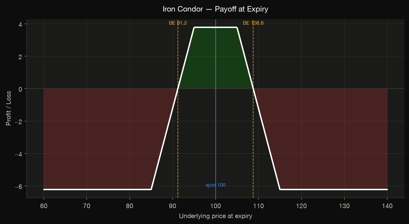
from jaxfolio.options import iron_condor, straddle, collar

condor = iron_condor(spot=100, put_long=85, put_short=95,
                     call_short=105, call_long=115, expiry=0.25, vol=0.22)

condor.net_premium()                 # + credit / − debit
condor.greeks(spot=100, vol=0.22)    # net delta / gamma / vega / theta / rho
condor.break_evens()                 # approximate break-even spot(s)
condor.payoff_at_expiry(spot_grid)   # P&L across terminal prices
condor.pnl_at(spot=102, vol=0.22, ttm_shift=1/12)   # mark-to-model at a horizon

Preset builders

Constructor	Structure
covered_call	long stock + short call (income, capped upside)
protective_put	long stock + long put (downside insurance)
collar	long stock + long put + short call (bounded, often ~zero cost)
bull_call_spread	long lower call + short upper call (capped bullish debit)
bear_put_spread	long upper put + short lower put (capped bearish debit)
straddle	long call + long put, same strike (large-move bet)
strangle	long OTM put + long OTM call (cheaper vol bet)
iron_condor	short strangle inside long wings (range-bound credit)
butterfly	1 / −2 / 1 calls (peak pinned at the middle strike)
calendar_spread	short near-dated + long far-dated call (theta/vega)

Calendar spreads

Because a calendar spread's legs have different expiries, analyze it with pnl_at (mark-to-model) rather than the at-expiry payoff.

Plotting payoffs and Greeks

from jaxfolio import viz

viz.save(viz.plot_payoff(condor, spot=100), "condor_payoff.png")
viz.save(viz.plot_greeks_profile(condor, spot=100, vol=0.22), "condor_greeks.png")

Profit shaded green, loss red; break-evens and spot annotated.

An implied-volatility surface, given a strike × expiry grid of IVs:

viz.save(viz.plot_vol_surface(spot, strikes, expiries, ivs), "surface.png")

Portfolio overlays

This is where the two halves of the library compose. The overlay module takes an optimizer's PortfolioResult and wraps the largest holdings in options, then aggregates the net Greeks and produces a combined payoff.

import jaxfolio as jf
from jaxfolio.options.overlay import collar_overlay, covered_call_overlay
import numpy as np

portfolio = jf.maximum_sharpe(returns)
spots = {a: 100.0 for a in portfolio.assets}

book = collar_overlay(portfolio, spots, top_n=5,
                      put_moneyness=0.95, call_moneyness=1.08,
                      expiry=0.25, vol=0.25)

book.net_greeks()                              # weighted net Greeks of the book
book.payoff_curve(np.linspace(0.7, 1.3, 200))  # weighted P&L across ±30% shocks

An OverlayBook holds the per-asset strategies scaled by portfolio weight; covered_call_overlay writes calls for income, collar_overlay bounds each holding between the put and call moneyness. Assets without a provided spot are skipped.

Volatility surfaces

A VolSurface turns a discrete grid of implied vols (strikes × expiries) into a smooth, callable iv(strike, ttm) by interpolating in total variance. Build one from market prices — which inverts each quote with the Newton implied_volatility solver — or fit a parametric raw-SVI slice per expiry.

import numpy as np
from jaxfolio.options import VolSurface

strikes = np.array([80, 90, 100, 110, 120.0])
ttms = np.array([0.1, 0.25, 0.5])
iv_grid = np.array([                          # one smile row per expiry
    [0.30, 0.25, 0.22, 0.24, 0.28],
    [0.29, 0.24, 0.21, 0.23, 0.27],
    [0.28, 0.23, 0.205, 0.225, 0.26],
])

surf = VolSurface.from_iv_grid(strikes, ttms, iv_grid, spot=100.0)
surf.iv(105, 0.3)                 # interpolated vol at an off-grid point
surf.price(105, 0.3)             # priced off the surface (reuses Black-Scholes)
surf.greeks(105, 0.3)            # full Greeks at the surface vol

fitted = surf.fit_svi()          # smooth, extrapolating raw-SVI smiles
surf.arbitrage_report()          # butterfly (convexity) + calendar checks

arbitrage_report() flags butterfly violations (call price must be convex in strike) and calendar violations (total variance must not decrease with maturity), so you can validate a surface before trading off it.

Discrete dividends & American exercise

binomial_american prices American-style options on a Cox–Ross–Rubinstein lattice with early exercise. It supports both a continuous dividend yield (div=) and a schedule of discrete cash dividends via the escrowed-dividend model:

from jaxfolio.options import binomial_american

# American put with a $3 cash dividend at 6 months (raises the put value):
binomial_american(100, 100, 1.0, 0.2, rate=0.05, is_call=False,
                  dividends=[(0.5, 3.0)])

Execution framework

Research simulation, not live trading

This simulates fills against a modeled Black–Scholes / surface price with transaction costs. It is a backtesting / research tool — not a live broker, order-management system, or exchange connection. Simulated fills, costs, and P&L will differ from live trading. See DISCLAIMER.md.

The jaxfolio.options.execution subpackage adds order/fill accounting, a transaction-CostModel, a mark-to-market option book, and an ExecutionSimulator. It is the options analogue of the walk-forward equity backtester:

import numpy as np
from jaxfolio.options.execution import (
    ExecutionSimulator, Instrument, Order, CostModel,
    simulate_covered_call_roll,
)

# Trade a single option with costs and mark the book to market.
sim = ExecutionSimulator(cost_model=CostModel(commission_per_contract=0.65,
                                              slippage_bps=5.0))
sim.execute(Order(Instrument("call", 105.0, 0.25), -1.0), spot=100.0, vol=0.2)
sim.book.net_greeks(100.0, 0.2)     # net position Greeks
sim.equity(100.0, 0.2)             # cash + mark-to-market book value

# Or roll a covered-call overlay through a whole price path.
path = 100 * np.cumprod(1 + np.random.default_rng(0).normal(0.0005, 0.01, 252))
res = simulate_covered_call_roll(path, moneyness=1.05, tenor=0.25,
                                 roll_every=21, vol=0.2)
res.total_return, res.stock_return, res.total_costs, res.n_rolls

simulate_covered_call_roll holds the underlying, writes a short call per share, and rolls it every roll_every steps — charging costs at each roll and returning the overlaid equity path alongside the buy-and-hold benchmark.