Multi-period optimization

Every other optimizer in jaxfolio is single-period. It collapses the return panel to \((\mu, \Sigma)\), emits one target weight vector, and knows nothing about what you currently hold. Transaction costs are then subtracted afterwards by the backtester, against a target that was chosen while blind to them.

The consequence is familiar: the optimizer says "sell half your largest position today", because nothing in its objective knows that trade is expensive.

multi_period_mean_variance answers a different and more actionable question — not "what should I hold?" but "what should I do today?" — by solving for the whole weight path at once, with costs priced inside the objective.

The problem

The variable is a \((T, N)\) matrix \(W\) whose row \(t\) is the portfolio to hold in period \(t\), anchored at the portfolio you hold now, \(w_0 \equiv w_{\text{prev}}\):

\[ \min_{W} \; \sum_{t=1}^{T} \Big[ \underbrace{-w_t^\top \mu_t + \tfrac{\gamma}{2}\, w_t^\top \Sigma_t w_t}_{\text{mean-variance, per period}} + \underbrace{c_{\text{lin}}^\top \lvert w_t - w_{t-1} \rvert}_{\text{spread + fees}} + \underbrace{c_{\text{quad}}^\top (w_t - w_{t-1})^2}_{\text{market impact}} \Big] \]

subject to every period independently satisfying the budget and bound constraints, \(\{w_t : \ell \le w_t \le u,\ \sum_i w_{t,i} = 1\}\).

The one thing to understand about costs

Linear costs alone will not produce a glide path. This surprises people, so it is worth being precise: a proportional cost creates a no-trade region — a band within which rebalancing is not worth the fee — but it gives no reason to split a trade, because moving from \(a\) to \(b\) in one step costs exactly the same as moving there in five. The optimum is to jump once to the cost-adjusted target and then hold.

Only quadratic market impact rewards spreading execution, because two half-sized trades cost half as much as one double-sized trade. That term is what turns the solution into a trajectory.

Both behaviors below are the exact optimum, confirmed against a CVXPY QP:

Costs	Planned turnover per period
50 bps linear only	0.442, 0.000, 0.000, 0.000, 0.000
10 bps linear + 500 bps impact	0.125, 0.092, 0.060, 0.030, 0.004

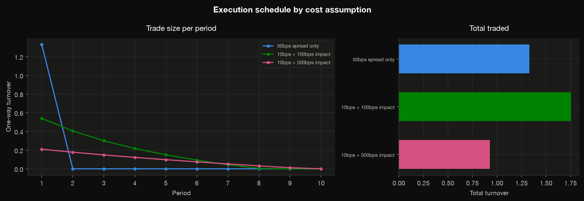
So: if you want execution scheduling, set impact_bps. If you only set spread_bps, you are asking for a turnover-penalized single-period portfolio, and that is what you will correctly get.

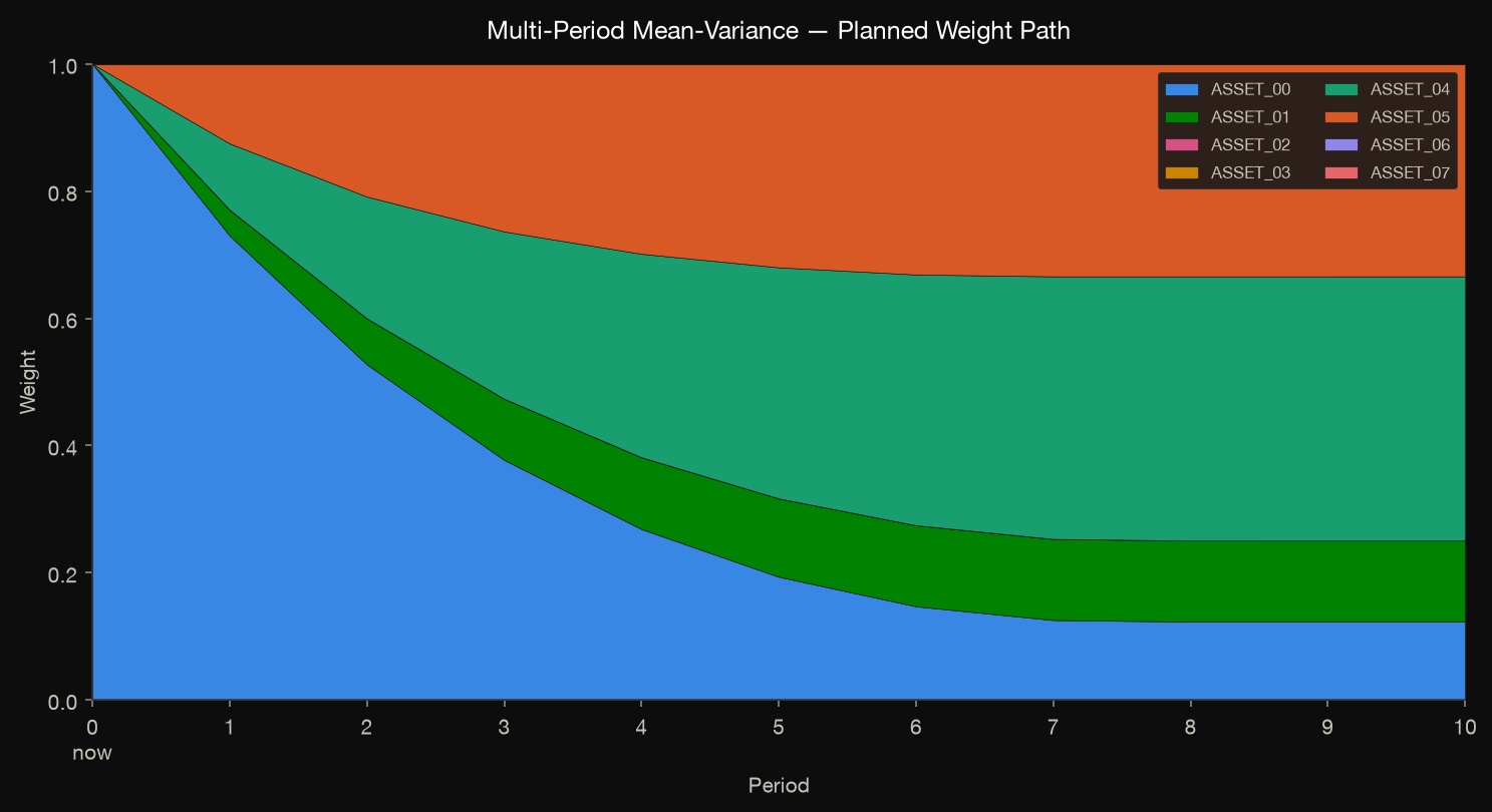
Unwinding a 100% single-name position over ten periods at 10 bps spread and 100 bps impact looks like this — the position bleeds down smoothly and the plan flattens as it converges, instead of gapping to the target on day one:

The cost model

TradingCosts collects the frictions. All three coefficients are quoted in basis points of traded notional per unit of \(\lvert \Delta w \rvert\), one-way, per period — the units a trader states them in — and each accepts a scalar or a per-asset sequence.

Field	Meaning
spread_bps	Bid-ask half-spread, linear in \(\lvert \Delta w \rvert\). A round trip costs 2 * spread_bps.
commission_bps	Proportional fee, also linear. Separate from the spread only for reporting.
impact_bps	Quadratic impact, per unit \((\Delta w)^2\). This is the term that spreads execution.
turnover_penalty	Extra L1 penalty in decimal units, for soft turnover control that is not a real cash cost.
smoothing	Numerical tuning knob — see accuracy below.

Costs are per period and never annualized: the objective trades them against per-period \(\mu\) and \(\Sigma\), so annualizing would double-count.

Usage

import jaxfolio as jf

returns = jf.generate_returns(n_assets=8, n_days=500, seed=42)
holdings = ...  # what you hold right now, aligned with jf.asset_columns(returns)

res = jf.multi_period_mean_variance(
    returns,
    horizon=5,
    w_prev=holdings,
    risk_aversion=3.0,
    costs=jf.TradingCosts(spread_bps=10.0, impact_bps=500.0),
)

res.weights                       # row 0 — trade into this today
res.trajectory                    # the full (5, 8) plan
res.metadata["turnover_path"]     # planned trade size per period
res.metadata["total_cost"]        # cost of executing the whole plan
res.metadata["terminal_weights"]  # the long-run target it is gliding toward

res.weights is the first row, not the last. That is what you act on, and it is what the backtester trades to. Under binding costs it sits close to w_prev, so res.sharpe describes your near-term holding and will look worse than a myopic single-period result — that is the honest reading, not a regression. For an apples-to-apples comparison use metadata["terminal_sharpe"].

w_prev defaults to a flat (all-zero) book, which correctly prices the cost of establishing a position. It need not sum to one.

A changing forecast

By default one \((\mu, \Sigma)\) from the panel is held across the horizon, so the trajectory is driven purely by costs. Pass a term structure to express a forecast that changes over the horizon:

res = jf.multi_period_mean_variance(
    returns, horizon=5, w_prev=holdings,
    mu_path=mu_t,     # (5, N)
    cov_path=cov_t,   # (5, N, N) — omit to reuse the sample covariance
)

Backtesting a path-aware strategy

The backtester supports these strategies through two additions, both of which are inert for every existing optimizer:

• Holdings injection. An optimizer that declares a w_prev keyword is handed the live portfolio at each rebalance. Detection is by signature, so a plain reference or a functools.partial both work.
• Trajectory execution. A returned trajectory is executed step by step over the following periods, paying cost on each step, instead of having every row but the first discarded. Disable with follow_trajectory=False to get the comparison arm.

from functools import partial
from jaxfolio.backtest import compare, metrics_table

results = compare(
    returns,
    {
        "myopic": partial(jf.mean_variance, risk_aversion=3.0),
        "multi-period": partial(
            jf.multi_period_mean_variance,
            horizon=5, risk_aversion=3.0,
            costs=jf.TradingCosts(spread_bps=50.0, impact_bps=500.0),
        ),
    },
    lookback=252, rebalance_every=21, transaction_cost=0.005,
)
metrics_table(results)[["annual_return", "sharpe", "avg_turnover", "total_cost"]]

examples/06_multiperiod_costs.py runs exactly this, and examples/notebooks/multiperiod.ipynb is the same story in notebook form.

A lambda hides the parameter

Holdings detection reads the signature, and lambda w: opt(w, w_prev=...) has the signature (w). Such a wrapper silently falls back to legacy behavior — which is the safe direction, but not what you wanted. Use functools.partial, pass the function directly, or force it with holdings_aware=True.

Two reporting notes. turnover is now indexed by trading period rather than rebalance (identical for path-less optimizers). And realized backtest turnover will not equal metadata["turnover_path"], because the plan assumes no drift whereas the engine lets weights drift with returns and then trades from the drifted book.

Visualizing a plan

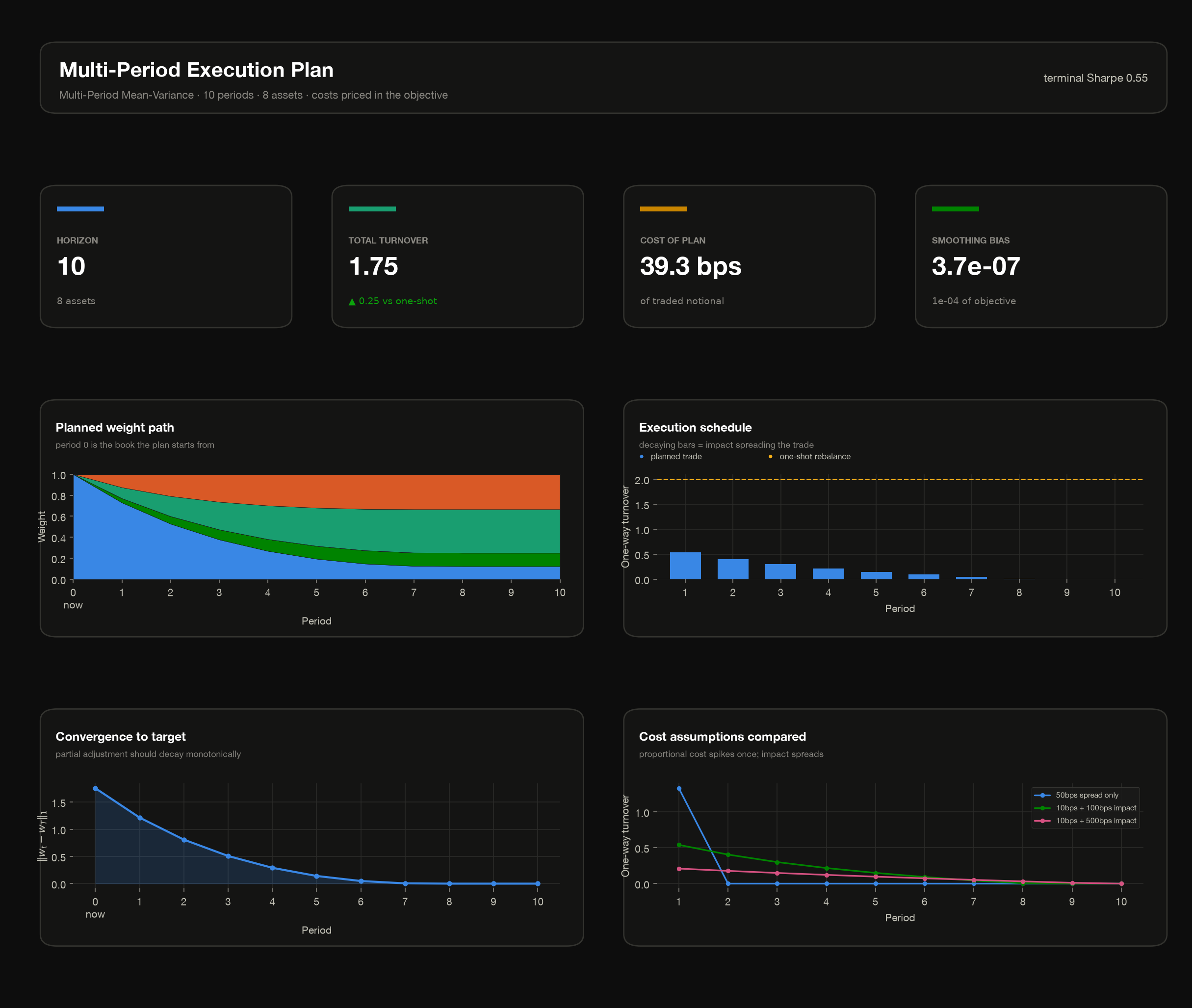
Five dedicated plots read a trajectory and its diagnostics directly — they label integer periods rather than dates, and anchor period 0 at the book the plan starts from. See the visualization guide.

from jaxfolio import viz

viz.plot_weight_path(res)                 # the trajectory
viz.plot_turnover_schedule(res)           # trade size per period + cumulative
viz.plot_path_convergence(res)            # distance to target; flags a short horizon
viz.plot_cost_comparison({...})           # schedules across cost assumptions
viz.multiperiod_dashboard(res)            # one-page report

Pass reference_weights= (the myopic optimum) to the schedule plot or the dashboard to see what the plan saves against a single rebalance. Without it no "one-shot" reference is drawn, deliberately: a monotone path's total turnover equals |w_T - w_prev| identically, so using the plan's own terminal weights would look like a comparison while measuring nothing.

Limitation: turnover caps are soft

Costs are priced, not capped. You can make turnover expensive; you cannot guarantee a turnover budget.

This is structural rather than an oversight. A hard cap \(\sum_t \lvert w_t - w_{t-1} \rvert \le \tau\) couples the periods, so the feasible set stops being a product of per-period sets — which is exactly the property that makes the projection a cheap row-wise operation. An exact projection onto \(\{\text{box} \cap \text{budget} \cap L_1\text{-ball}\}\) would need Dykstra or ADMM: a second solver with its own tuning and stopping rule, reusing none of the existing machinery.

If you have a genuine compliance limit, raise spread_bps / turnover_penalty until metadata["total_turnover"] sits under it, and verify per rebalance. Do not represent the result as a guaranteed cap.

Accuracy

The \(L_1\) trade cost is non-differentiable exactly where the optimum sits — at zero trade, for every asset that should not move. Applied directly, a first-order method stalls around 1% above the true optimum regardless of solver family; this is the same failure mode that limits min_cvar.

The optimizer therefore Huber-smooths the term. Because accuracy turns out not to be monotone in the smoothing width, it walks a ladder of shrinking widths and keeps whichever iterate scores best under the exact, un-smoothed objective. Measured against a tightly converged CVXPY QP across 4–50 assets and six cost regimes, that selection takes the worst-case relative gap from 8–160% down to 2e-4, with a typical gap near 1e-6. Frictionless and impact-dominated problems land at ~1e-8; the stiff case is a mid-range linear cost, where the \(L_1\) term rivals the entire mean-variance curvature.

Diagnostics that let you audit this per solve:

Key	Meaning
smoothing_bias	objective_exact - objective_smoothed, i.e. how much the Huber band understated the true cost. Non-negative.
selected_stage	Which ladder rung won. -1 means the no-trade path was never beaten, which is correct under high costs.
stage_objective_exact	The exact objective at every rung, so the selection is inspectable.
residual / converged	Projected-gradient norm at the chosen iterate.

converged: False is not necessarily a failure

When the linear cost is large relative to the smoothing width, the residual legitimately plateaus far above tol while the answer is exactly right — the correct action is "do not trade", and the residual is carrying the un-actioned cost gradient. Judge the solve on smoothing_bias and the objective, not on this flag alone.

Performance

One compilation is spent per distinct (horizon, n_assets) pair, because the horizon is baked into the variable's shape. Sweeping costs or risk_aversion is free — every cost travels as a traced parameter — but varying horizon per rebalance in a backtest recompiles each time.

The ladder self-adapts to difficulty: an impact-dominated problem converges in a few dozen iterations, while a stiff linear-cost problem may spend tens of thousands.