Backtesting

The backtester is a vectorized walk-forward engine that is completely optimizer-agnostic: it accepts any callable optimizer(window) → PortfolioResult — built-in, custom, or a partially-applied variant — rebalances on a fixed schedule, applies linear transaction costs on turnover, and lets weights drift with returns between rebalances.

How the walk-forward works

At each step \(t\) beyond the initial lookback:

1. Rebalance (every rebalance_every periods): hand the trailing lookback window to the optimizer, align its weights to the panel's asset order, and charge transaction_cost × turnover, where turnover is the \(\ell_1\) change \(\sum_i |w^{\text{target}}_i - w^{\text{current}}_i|\).
2. Accrue the period return net of any cost: \(r^{\text{strat}}_t = w^\top r_t - \text{cost}\).
3. Drift the weights with realized returns between rebalances (buy-and-hold), renormalizing so they continue to sum to one.

This avoids look-ahead bias — the optimizer only ever sees data strictly before the period it is allocating for.

Single backtest

from jaxfolio.backtest import backtest
import jaxfolio as jf

returns = jf.generate_returns(n_assets=12, n_days=1000, seed=11)

result = backtest(
    returns,
    jf.maximum_sharpe,
    name="Max Sharpe",
    lookback=252,            # trailing window handed to the optimizer
    rebalance_every=21,      # ≈ monthly for daily data
    transaction_cost=0.0010, # 10 bps per unit of one-way turnover
    risk_free=0.0,
)

backtest returns a BacktestResult holding the net-of-cost return series, the full weight history, turnover, and a metrics summary:

result.returns          # pd.Series of net strategy returns
result.weights          # pd.DataFrame — dates × assets
result.turnover         # pd.Series
result.metrics          # dict of headline metrics
result.equity_curve     # cumulative growth of $1
result.drawdown         # underwater curve

Comparing several strategies

compare runs the same backtest across a {name: optimizer} map (all keyword arguments are forwarded), and metrics_table assembles a tidy comparison frame:

from jaxfolio.backtest import compare, metrics_table

results = compare(returns, {
    "1/N":            jf.equal_weight,
    "Min Variance":   jf.minimum_variance,
    "Max Sharpe":     jf.maximum_sharpe,
    "Risk Parity":    jf.risk_parity,
    "HRP":            jf.hierarchical_risk_parity,
    "MST Centrality": jf.mst_centrality,
    "Online EG":      jf.online_gradient,
}, lookback=252, rebalance_every=21, transaction_cost=0.0010)

table = metrics_table(results)[
    ["annual_return", "annual_volatility", "sharpe", "max_drawdown", "avg_turnover"]
]
print(table.round(3).to_string())

Backtesting a parameterized method

Optimizers that take extra arguments (views, alpha, an LLM client) need those bound first. Use functools.partial:

from functools import partial
compare(returns, {
    "MV (γ=5)":  partial(jf.mean_variance, risk_aversion=5.0),
    "CVaR 99%":  partial(jf.min_cvar, alpha=0.99),
})

Metrics

The metrics module computes every statistic from a periodic return series; summary bundles the headline set that the backtester attaches to each result.

Metric	Meaning
annual_return	Geometric annualized return (CAGR)
annual_volatility	Annualized standard deviation
sharpe	Annualized Sharpe ratio
sortino	Sharpe with a downside-deviation denominator
max_drawdown	Largest peak-to-trough decline (negative)
calmar	Annual return ÷ |max drawdown|
var_95	Historical Value-at-Risk at 95% (a positive loss)
cvar_95	Historical expected shortfall at 95%
hit_rate	Fraction of periods with a positive return
avg_turnover	Mean one-way turnover per rebalance

Each is also callable directly on any return series:

from jaxfolio.backtest import metrics

metrics.sharpe_ratio(result.returns, risk_free=0.0)
metrics.max_drawdown(result.returns)
metrics.conditional_value_at_risk(result.returns, alpha=0.99)

Visualizing the run

from jaxfolio import viz

viz.save(viz.plot_equity_curves(results), "equity.png")
viz.save(viz.plot_drawdown(results), "drawdown.png")
viz.save(viz.dashboard(results, returns), "dashboard.png")

Cumulative growth of $1, direct-labeled per strategy.

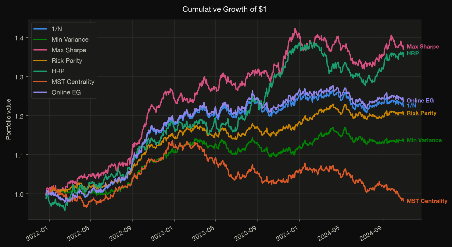
See the Visualization guide for the full plot catalog.