Optimizers

Every optimizer shares the interface method(returns, ...) → PortfolioResult and — for the constrained classical methods — the same projected-gradient solver. This guide states each method's objective, its parameters, and the diagnostics it records, grouped into four families.

Throughout, \(w \in \mathbb{R}^N\) is the weight vector, \(\mu\) the vector of expected (per-period) returns, and \(\Sigma\) the return covariance matrix. Unless noted, the feasible set is the long-only simplex \(\{w : w \ge 0,\ \sum_i w_i = 1\}\), configurable through OptimizerConfig.

The catalog

Family	Methods
Baselines	equal_weight, inverse_volatility
Classical (solver)	minimum_variance, mean_variance, maximum_sharpe, maximum_diversification, risk_parity, kelly, min_cvar, black_litterman
Learning	deep_sharpe, online_gradient
Graph	hierarchical_risk_parity, hierarchical_equal_risk, mst_centrality

---

Baselines

Cheap, closed-form weightings that are famously hard to beat and make honest benchmarks in any comparison.

equal_weight

The \(1/N\) portfolio: \(w_i = 1/N\). No estimation, no error — the reference every other method must justify beating.

jf.equal_weight(returns)

inverse_volatility

Naive risk parity — weight inversely to each asset's own volatility, ignoring correlations:

\[ w_i \propto \frac{1}{\sqrt{\Sigma_{ii}}}, \qquad \sum_i w_i = 1. \]

jf.inverse_volatility(returns)

---

Classical optimizers

These minimize a differentiable objective under the configured constraints with the shared solver. Each accepts an optional config: OptimizerConfig.

minimum_variance

The global minimum-variance portfolio:

\[ \min_{w \in \mathcal{C}}\; w^\top \Sigma\, w \;+\; \lambda_{2}\lVert w \rVert_2^2 . \]

The optional \(\ell_2\) term (config.l2_reg) discourages concentration.

jf.minimum_variance(returns)

mean_variance

Markowitz mean–variance utility with risk-aversion \(\gamma\):

\[ \max_{w \in \mathcal{C}}\; w^\top \mu \;-\; \tfrac{\gamma}{2}\, w^\top \Sigma\, w . \]

Larger risk_aversion tilts toward lower variance.

jf.mean_variance(returns, risk_aversion=1.0)

maximum_sharpe

The tangency portfolio — maximum Sharpe ratio:

\[ \max_{w \in \mathcal{C}}\; \frac{w^\top \mu - r_f}{\sqrt{w^\top \Sigma\, w}} . \]

The Sharpe ratio is scale-invariant, so the problem is optimized directly on the simplex. config.risk_free_rate sets the per-period \(r_f\).

jf.maximum_sharpe(returns)

maximum_diversification

Maximizes the diversification ratio (Choueifaty & Coignard, 2008) — the ratio of the weighted-average asset volatility to the portfolio volatility:

\[ \max_{w \in \mathcal{C}}\; \frac{w^\top \sigma}{\sqrt{w^\top \Sigma\, w}}, \qquad \sigma_i = \sqrt{\Sigma_{ii}} . \]

jf.maximum_diversification(returns)

risk_parity

The equal-risk-contribution (ERC) portfolio: each asset contributes equally to total portfolio risk. Solved with the cyclical coordinate descent of Griveau-Billion, Richard & Roncalli (2013) on the convex program

\[ \min_{x > 0}\; \tfrac12\, x^\top \Sigma\, x - \frac{1}{N}\sum_i \log x_i, \]

whose normalized fixed point \(w = x / \sum_i x_i\) equalizes the risk contributions \(w_i (\Sigma w)_i\). Each coordinate update is a one-dimensional quadratic solved in closed form, keeping \(x_i\) strictly positive and converging regardless of covariance scale.

result = jf.risk_parity(returns)
result.metadata["risk_contributions"]   # per-asset, equalized at 1/N

The realized risk contributions are stored in metadata — plot them with plot_risk_contributions.

kelly

The growth-optimal (log-wealth) portfolio, maximizing expected log-growth over the sample paths:

\[ \max_{w \in \mathcal{C}}\; \frac{1}{T}\sum_{t=1}^{T} \log\!\bigl(1 + w^\top r_t\bigr) . \]

Optimized over the return matrix directly (not just its moments).

jf.kelly(returns)

min_cvar

Minimum Conditional-Value-at-Risk (Rockafellar & Uryasev, 2000). Using the auxiliary-variable formulation, weights \(w\) and the VaR threshold \(\tau\) are optimized jointly:

\[ \min_{w \in \mathcal{C},\, \tau}\; \tau + \frac{1}{(1-\alpha)\,T} \sum_{t=1}^{T}\bigl[\,\ell_t - \tau\,\bigr]_+, \qquad \ell_t = -\,w^\top r_t . \]

result = jf.min_cvar(returns, alpha=0.95)
result.metadata["cvar"], result.metadata["var"]

black_litterman

Blends the market-implied equilibrium with your own views. Reverse optimization gives the equilibrium (prior) excess returns \(\pi = \gamma\,\Sigma\, w_{\text{mkt}}\); absolute views \(P w = q\) with uncertainty \(\Omega\) yield the He & Litterman posterior mean

\[ \bar\mu = \bigl[(\tau\Sigma)^{-1} + P^\top \Omega^{-1} P\bigr]^{-1} \bigl[(\tau\Sigma)^{-1}\pi + P^\top \Omega^{-1} q\bigr], \]

which is then mean–variance optimized. With no views, the result reduces to the equilibrium (market) portfolio.

result = jf.black_litterman(
    returns,
    views={"ASSET_00": 0.02, "ASSET_03": -0.01},   # absolute per-period views
    view_confidence=0.5,                            # (0, 1] — higher = tighter
    tau=0.05,
    risk_aversion=2.5,
)
result.metadata["posterior_returns"]

LLM-generated views

black_litterman is the engine behind the LLM strategies: a local model produces the views and a dispersion-calibrated view_confidence.

---

Learning-based

Differentiable and online methods — the ones that only exist because the whole pipeline is JAX.

deep_sharpe

An end-to-end differentiable allocation policy. A small MLP maps the flattened trailing lookback window of returns to long-only weights (via softmax), trained by gradient ascent to maximize the annualized Sharpe of the strategy's realized returns across all windows. Pure JAX + optax — no flax dependency. The reported allocation is the policy applied to the most recent window; the trained parameters are retained in metadata so the policy can be rolled forward.

\[ \max_{\theta}\;\; \sqrt{P}\cdot \frac{\operatorname{mean}_t \, r^{\text{strat}}_t(\theta)} {\operatorname{std}_t \, r^{\text{strat}}_t(\theta)}, \qquad w_t(\theta) = \operatorname{softmax}\bigl(\text{MLP}_\theta(\text{window}_t)\bigr). \]

result = jf.deep_sharpe(returns, lookback=60, hidden=(64, 32), epochs=300, seed=0)
result.metadata["final_train_sharpe"], result.metadata["params"]

online_gradient

The exponentiated-gradient (EG) universal online portfolio (Helmbold et al.). Weights update multiplicatively by realized returns, achieving sub-linear regret versus the best constant-rebalanced portfolio in hindsight:

\[ w_{t+1,i} \;\propto\; w_{t,i}\, \exp\!\left(\eta\, \frac{r_{t,i}}{w_t^\top r_t}\right). \]

result = jf.online_gradient(returns, eta=0.05)
result.metadata["final_wealth"], result.metadata["wealth_path"]

---

Graph-based

Hierarchy- and network-based allocation. These are combinatorial (SciPy linkage / MST) rather than gradient-based.

hierarchical_risk_parity

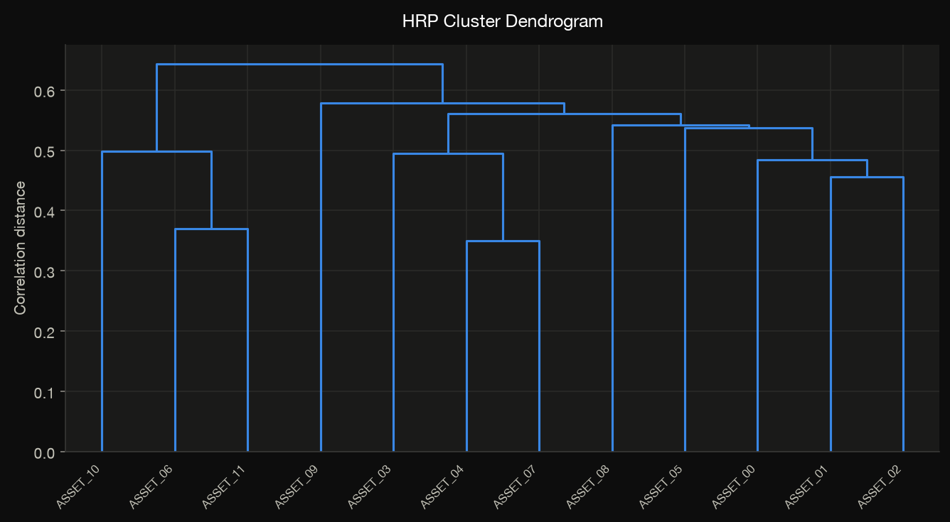
López de Prado's HRP (2016). Cluster assets by the correlation-distance \(d_{ij} = \sqrt{\tfrac12 (1 - \rho_{ij})}\) dendrogram, quasi-diagonalize the covariance by the leaf order, then recursively bisect and split capital by inverse cluster variance. Robust to the ill-conditioned covariances that break classical mean–variance.

result = jf.hierarchical_risk_parity(returns, linkage_method="single")
result.metadata["linkage"]   # feeds plot_dendrogram

The HRP linkage tree via viz.plot_dendrogram.

hierarchical_equal_risk

HERC — cut the dendrogram into n_clusters groups, allocate across clusters by inverse cluster variance and within each cluster by inverse variance. A more robust, less order-sensitive cousin of HRP.

jf.hierarchical_equal_risk(returns, n_clusters=4, linkage_method="ward")

mst_centrality

Build the minimum spanning tree of the correlation-distance network; assets with lower degree centrality (more peripheral, less coupled to the market core) receive more weight:

\[ w_i \;\propto\; \frac{1}{(\deg_i)^{\alpha}} . \]

Eigenvector centrality and the MST adjacency are recorded in metadata for the correlation-network plot.

jf.mst_centrality(returns, alpha=1.0)

---

Choosing a method

If you want…	Consider
An honest benchmark	equal_weight, inverse_volatility
Lowest risk	minimum_variance, risk_parity
Best risk-adjusted return	maximum_sharpe, mean_variance
Tail-risk control	min_cvar
To express a subjective view	black_litterman
Robustness to noisy covariances	hierarchical_risk_parity, hierarchical_equal_risk
Growth maximization	kelly
A learned, adaptive policy	deep_sharpe, online_gradient

Then compare them fairly with a walk-forward backtest — the in-sample optimum is rarely the out-of-sample winner.