Quickstart

This page walks the full workflow end to end — data in, allocation out, compared and visualized — in a few minutes. Every snippet runs offline against reproducible synthetic data.

1. Get some returns

Any wide, date-by-asset returns panel works: a pandas DataFrame, a NumPy array, or the built-in synthetic generator. Start with synthetic data so the results are reproducible:

import jaxfolio as jf

returns = jf.generate_returns(n_assets=10, n_days=756, seed=7)
returns.shape          # (755, 10) — one row per day, one column per asset

To use real data instead, swap in a loader (requires the data extra):

returns = jf.to_returns(jf.load_yfinance(["AAPL", "MSFT", "NVDA", "JPM"]))

See the Data guide for CSV, Parquet, and Yahoo Finance loaders.

2. Optimize

Every optimizer shares the same shape — method(returns) → PortfolioResult:

result = jf.maximum_sharpe(returns)

result.sharpe            # annualized Sharpe ratio
result.expected_return   # annualized expected return
result.volatility        # annualized volatility
result.top(3)            # {'ASSET_04': 0.31, 'ASSET_01': 0.22, ...}

A PortfolioResult carries the weights, the asset names, annualized diagnostics, and a free-form metadata dict (iteration counts, cluster labels, posterior returns, and so on — depending on the method).

Swap the method name to try another approach — the call site does not change:

jf.minimum_variance(returns)
jf.risk_parity(returns)
jf.hierarchical_risk_parity(returns)
jf.black_litterman(returns, views={"ASSET_00": 0.02})

See the Optimizers guide for all sixteen methods and their mathematics.

3. Compare with a walk-forward backtest

compare runs a walk-forward backtest — rolling window, periodic rebalance, linear transaction costs — for several optimizers on the same data:

from jaxfolio.backtest import compare, metrics_table

results = compare(returns, {
    "Max Sharpe":  jf.maximum_sharpe,
    "HRP":         jf.hierarchical_risk_parity,
    "Risk Parity": jf.risk_parity,
    "1/N":         jf.equal_weight,
}, lookback=252, rebalance_every=21, transaction_cost=0.0010)

print(metrics_table(results).round(3))

metrics_table returns a tidy pandas frame of net-of-cost performance and risk metrics (annual return, volatility, Sharpe, Sortino, Calmar, max drawdown, VaR, CVaR, hit rate, and average turnover). See the Backtesting guide.

4. Visualize

The viz module returns matplotlib figures on a validated dark theme. The composite dashboard bundles the headline story into one report:

from jaxfolio import viz

highlight = {
    "Max Sharpe":   jf.maximum_sharpe(returns),
    "Min Variance": jf.minimum_variance(returns),
    "HRP":          jf.hierarchical_risk_parity(returns),
}

fig = viz.dashboard(results, returns, highlight=highlight)
viz.save(fig, "dashboard.png")

KPI strip, equity curves, drawdown, efficient frontier, and a Sharpe ranking.

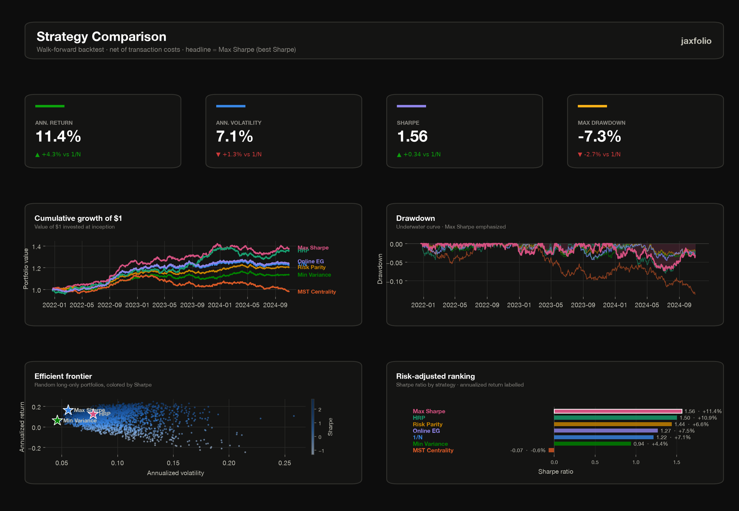
Individual plots are one call each:

viz.save(viz.plot_efficient_frontier(returns, highlight=highlight), "frontier.png")
viz.save(viz.plot_equity_curves(results), "equity.png")
viz.save(viz.plot_weights(result), "weights.png")

See the Visualization guide for the full catalog.

5. Add an options overlay (optional)

The optimizer output composes directly with the options layer — for example, writing protective collars over the largest holdings:

from jaxfolio.options.overlay import collar_overlay

portfolio = jf.maximum_sharpe(returns)
spots = {a: 100.0 for a in portfolio.assets}       # reference spot per asset

book = collar_overlay(portfolio, spots, top_n=5,
                      put_moneyness=0.95, call_moneyness=1.08)

book.net_greeks()                                  # net delta / gamma / vega / theta / rho

See the Options guide.

Where to go next

Core concepts

The shared solver, PortfolioResult, and the moment pipeline.

Optimizers

All sixteen methods with their objectives and constraints.

Custom strategies

Author your own method with the toolkit building blocks.